One of Cosmic Frog’s great competitive features is the ability to quickly run many sensitivity analysis scenarios in parallel on Optilogic’s Cloud-based platform. This built-in Sensitivity at Scale (S@S) functionality lets a user run sensitivity on demand quantity and transportation costs with 1 click of a button, on any scenario using any of Cosmic Frog’s engines. In this documentation, we will walk through how to kick-off a S@S run, where to track the status of the scenarios, and show some example outputs of S@S scenarios once they have completed running.
Kicking off a S@S analysis is simply done by clicking on the green S@S button on the right-hand side in the toolbar at the top of Cosmic Frog:

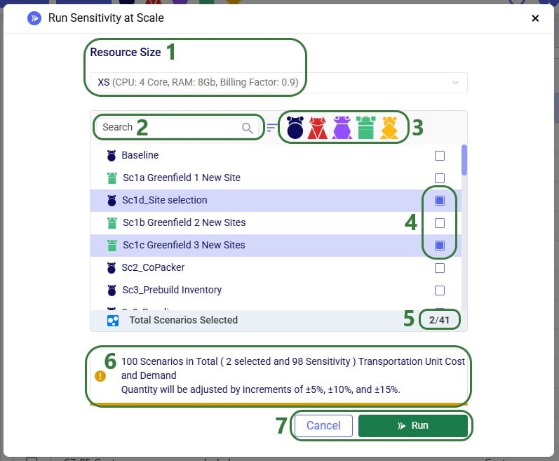
After clicking on the S@S button, the Run Sensitivity at Scale screen comes up:
Please note that the parameters that are configured on the Run Settings screen (which comes up when clicking on the Run button at the right top of Cosmic Frog) are used for the Sensitivity at Scale scenario runs.
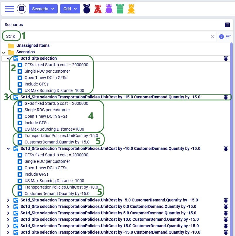
The scenarios are then created in the model, and we can review their setup by switching to the Scenarios module within Cosmic Frog:
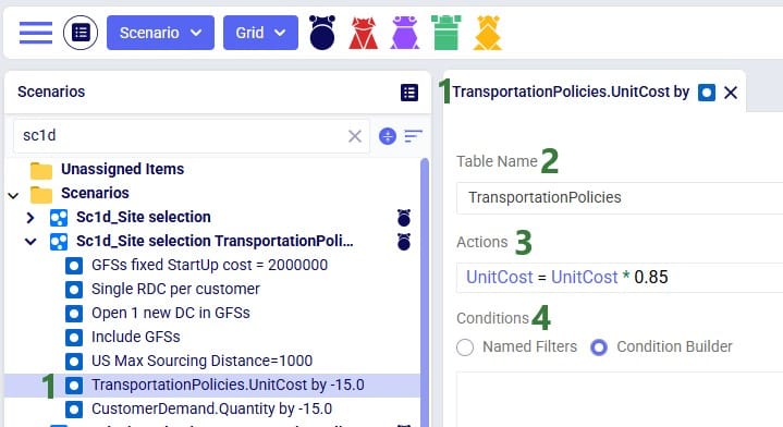
As an example of the sensitivity scenario items that are being created and assigned to the sensitivity scenarios as part of the S@S process, let us have a look at one of these newly created scenario items:
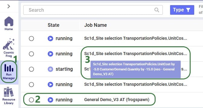
Once the sensitivity scenarios have been created, they are kicked off to all be run simultaneously. Users can have a look in the Run Manager application on the Optilogic platform to track their progress:
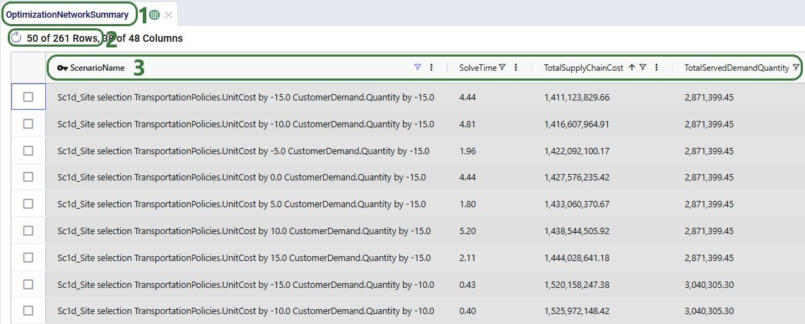
Once a S@S scenario finishes, its outputs are available for review in Cosmic Frog. As with other models and scenarios, users can review outputs through output tables, maps, and graphs/charts/dashboards in the Analytics module. Here we will just show the Optimization Network Summary output table and a cost comparison chart as example outputs. Depending on the model and technology run, users may want to look at different outputs to best understand them.
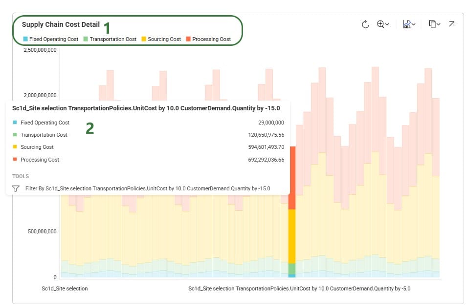
To understand how the costs are divided over the different cost types and how they compare by scenario, we can look at following Supply Chain Cost Detail graph in the Analytics module:
One of Cosmic Frog’s great competitive features is the ability to quickly run many sensitivity analysis scenarios in parallel on Optilogic’s Cloud-based platform. This built-in Sensitivity at Scale (S@S) functionality lets a user run sensitivity on demand quantity and transportation costs with 1 click of a button, on any scenario using any of Cosmic Frog’s engines. In this documentation, we will walk through how to kick-off a S@S run, where to track the status of the scenarios, and show some example outputs of S@S scenarios once they have completed running.
Kicking off a S@S analysis is simply done by clicking on the green S@S button on the right-hand side in the toolbar at the top of Cosmic Frog:
After clicking on the S@S button, the Run Sensitivity at Scale screen comes up:
Please note that the parameters that are configured on the Run Settings screen (which comes up when clicking on the Run button at the right top of Cosmic Frog) are used for the Sensitivity at Scale scenario runs.
The scenarios are then created in the model, and we can review their setup by switching to the Scenarios module within Cosmic Frog:
As an example of the sensitivity scenario items that are being created and assigned to the sensitivity scenarios as part of the S@S process, let us have a look at one of these newly created scenario items:
Once the sensitivity scenarios have been created, they are kicked off to all be run simultaneously. Users can have a look in the Run Manager application on the Optilogic platform to track their progress:
Once a S@S scenario finishes, its outputs are available for review in Cosmic Frog. As with other models and scenarios, users can review outputs through output tables, maps, and graphs/charts/dashboards in the Analytics module. Here we will just show the Optimization Network Summary output table and a cost comparison chart as example outputs. Depending on the model and technology run, users may want to look at different outputs to best understand them.
To understand how the costs are divided over the different cost types and how they compare by scenario, we can look at following Supply Chain Cost Detail graph in the Analytics module: